Basic Linear Algebra
Vectors
A vector is a list of numbers.
\[\mathbf{a} = \begin{pmatrix} a_1 \\ a_2 \\ \vdots \\ a_n \end{pmatrix}\]
where \(a_i\) is the \(i\)-th element of the vector. A vector is often denoted by a bold letter, such as \(\mathbf{a}\). A vector with \(n\) elements is called an \(n\)-dimensional vector. We also call it a (\(n \times 1\)) vector.
Magnitude of a Vector
The magnitude of a (\(n \times 1\)) vector \(\mathbf{a}\) is defined as the square root of the sum of the squares of the elements of \(\mathbf{a}\).
\[\|\mathbf{a}\| = \sqrt{\mathbf{a}^\top \mathbf{a}} = \sqrt{\sum_{i=1}^{n} a_i^2}\]
Don’t worry about \(\mathbf{a}^\top \mathbf{a}\) for now. It’s just a compact form of the sum of the squares of the elements of \(\mathbf{a}\). We will cover it in more detail later.
Unit Vector
A unit vector is a vector with a magnitude of 1.
\[\|\mathbf{u}\| = 1\]
where \(\mathbf{u}\) is a (\(n \times 1\)) vector and \(\|\mathbf{u}\|\) is the magnitude of \(\mathbf{u}\).
We can turn every (\(n \times 1\)) vector into a unit vector by dividing the vector by its magnitude:
\[\mathbf{u} = \frac{\mathbf{a}}{\|\mathbf{a}\|}\]
- Note that it doesn’t change the direction of the vector.
Inner Product
The inner product of two vectors \(\mathbf{a}\) (\(n \times 1\)) and \(\mathbf{b}\) (\(n \times 1\)) is defined as:
\[\mathbf{a} \cdot \mathbf{b} = \mathbf{a}^\top \mathbf{b} = \sum_{i=1}^{n} a_i b_i\]
- It is also known as the dot product.
- The result is a scalar.
- It is symmetric: \(\mathbf{a} \cdot \mathbf{b} = \mathbf{b} \cdot \mathbf{a}\).
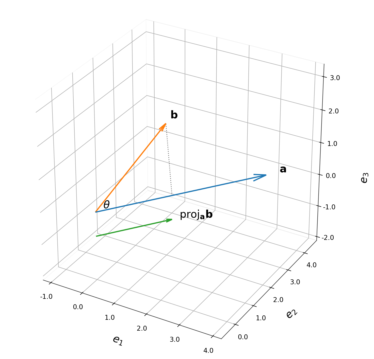
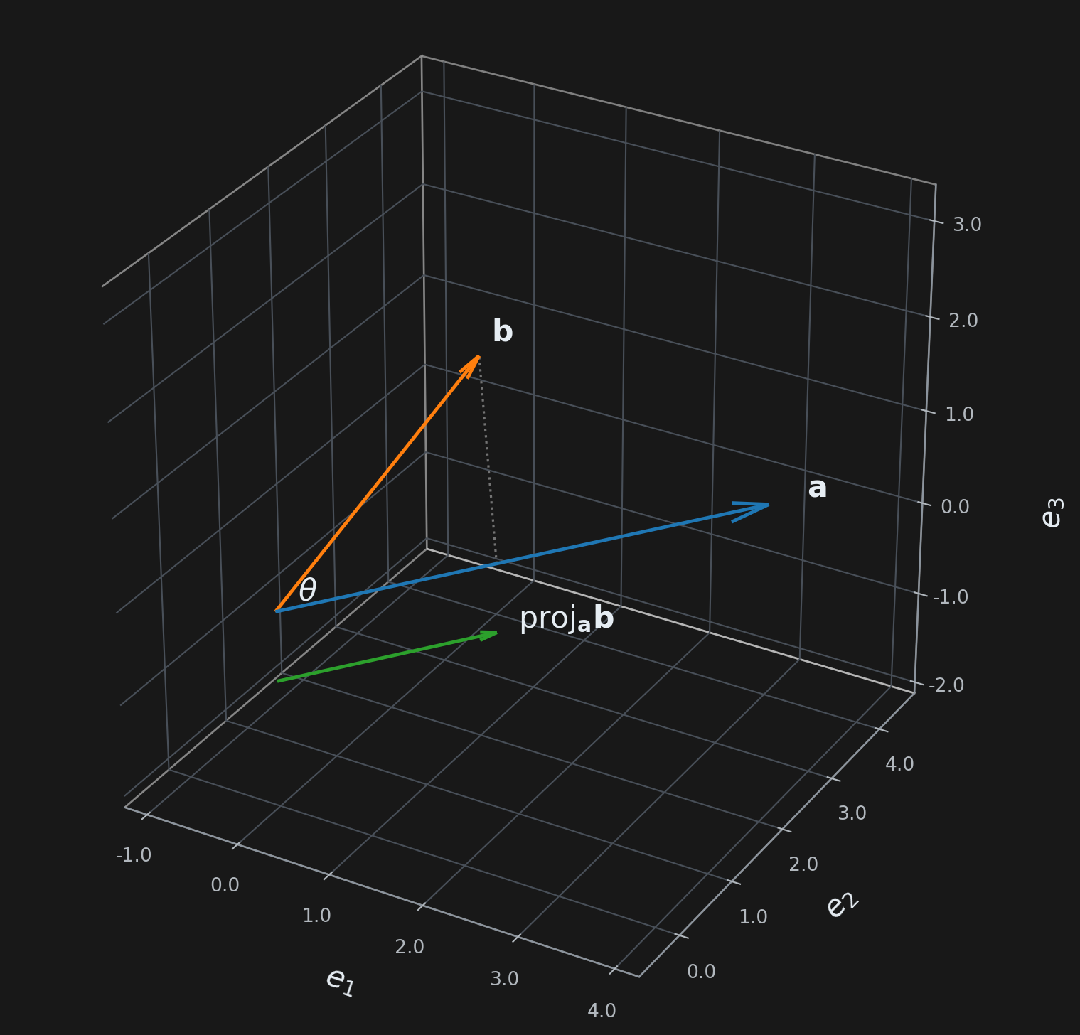
- If \(\mathbf{a}\) is a unit vector, then \(\mathbf{a} \cdot \mathbf{b}\) is the projection of \(\mathbf{b}\) onto \(\mathbf{a}\).
Angle Between Two Vectors
The angle between two vectors \(\mathbf{a}\) and \(\mathbf{b}\) is defined as:
\[\theta = \cos^{-1} \left( \frac{\mathbf{a} \cdot \mathbf{b}}{\|\mathbf{a}\| \|\mathbf{b}\|} \right)\]
Outer Product
The outer product of two vectors \(\mathbf{a}\) (\(m \times 1\)) and \(\mathbf{b}\) (\(n \times 1\)) is defined as:
\[\mathbf{a} \otimes \mathbf{b} = \mathbf{a} \mathbf{b}^\top\]
- The result is an \(m \times n\) matrix.
- It is not symmetric: \(\mathbf{a} \otimes \mathbf{b} \neq \mathbf{b} \otimes \mathbf{a}\).
Matrices
A matrix is a rectangular array of numbers.
\[A = \begin{pmatrix} a_{11} & a_{12} & \cdots & a_{1n} \\ a_{21} & a_{22} & \cdots & a_{2n} \\ \vdots & \vdots & \ddots & \vdots \\ a_{m1} & a_{m2} & \cdots & a_{mn} \end{pmatrix}\]
where \(a_{ij}\) is the element in the \(i\)-th row and \(j\)-th column of the matrix. A matrix is often denoted by a capital letter, such as \(A\). A matrix with \(m\) rows and \(n\) columns is called an \(m \times n\) matrix. We also call it a (\(m \times n\)) matrix.
Matrix Multiplication
The product of two matrices \(A\) (\(m \times n\)) and \(B\) (\(n \times p\)) is defined as:
\[C = AB\]
where \(C\) is a (\(m \times p\)) matrix.
The element in the \(i\)-th row and \(j\)-th column of \(C\) is given by the inner product of the \(i\)-th row of \(A\) and the \(j\)-th column of \(B\):
\[c_{ij} = \sum_{k=1}^{n} a_{ik} b_{kj}\]
Rank of a Matrix
The rank of a matrix is the maximum number of linearly independent rows or columns in the matrix. Equivalently, it equals the dimension of the vector space spanned by its rows (or columns).
Key Ideas
- Linear independence means no row (or column) can be expressed as a linear combination of the others.
- The row rank always equals the column rank — this is a fundamental theorem of linear algebra.
- For an \(m \times n\) matrix, the rank is at most \(\min(m, n)\).
How to Find the Rank
The standard method is Gaussian elimination (row reduction to row echelon form). The rank equals the number of non-zero rows (pivot rows) after reduction.
Example:
\[A = \begin{bmatrix} 1 & 2 & 3 \\ 2 & 4 & 6 \\ 0 & 1 & 2 \end{bmatrix}\]
Row 2 is exactly \(2 \times\) Row 1, so it’s linearly dependent. After reduction, only 2 non-zero rows remain → \(\operatorname{rank}(A) = 2\).
Special Cases
| Situation | Rank |
|---|---|
| Zero matrix | \(0\) |
| Identity matrix \(I_n\) | \(n\) |
| Full rank (all rows/cols independent) | \(\min(m, n)\) |
| Rank-deficient (rows/cols are dependent) | \(< \min(m, n)\) |
Why It Matters
The rank reveals important properties of a linear system \(A\mathbf{x} = \mathbf{b}\):
- Unique solution → \(A\) is square and full rank.
- No solution or infinitely many → \(A\) is rank-deficient.
- The rank determines the dimensions of the null space (via the rank-nullity theorem: \(\text{rank} + \text{nullity} = n\)).
In short, the rank tells you how much “true information” or “dimensionality” a matrix contains.
Determinant
2×2 Matrix
\[\det(A) = \begin{vmatrix} a & b \\ c & d \end{vmatrix} = ad - bc\]
3×3 Matrix (cofactor expansion)
\[\det(A) = \begin{vmatrix} a & b & c \\ d & e & f \\ g & h & i \end{vmatrix} = a\begin{vmatrix} e & f \\ h & i \end{vmatrix} - b\begin{vmatrix} d & f \\ g & i \end{vmatrix} + c\begin{vmatrix} d & e \\ g & h \end{vmatrix}\]
Which expands to:
\[\det(A) = a(ei - fh) - b(di - fg) + c(dh - eg)\]
Cofactor expansion along row \(i\)
\[\det(A) = \sum_{j=1}^{n} (-1)^{i+j} \, a_{ij} \, M_{ij}\]
where \(M_{ij}\) is the minor — the determinant of the submatrix formed by deleting row \(i\) and column \(j\).
Diagonal and triangular matrices shortcut
For a diagonal matrix \(A\): \[A = \begin{pmatrix} a_{11} & 0 & \cdots & 0 \\ 0 & a_{22} & \cdots & 0 \\ \vdots & \vdots & \ddots & \vdots \\ 0 & 0 & \cdots & a_{nn} \end{pmatrix}\]
Or for a lower triangular matrix \(A\): \[A = \begin{pmatrix} a_{11} & 0 & \cdots & 0 \\ a_{21} & a_{22} & \cdots & 0 \\ \vdots & \vdots & \ddots & \vdots \\ a_{n1} & a_{n2} & \cdots & a_{nn} \end{pmatrix}\]
Or for an upper triangular matrix \(A\):
\[A = \begin{pmatrix} a_{11} & a_{12} & \cdots & a_{1n} \\ 0 & a_{22} & \cdots & a_{2n} \\ \vdots & \vdots & \ddots & \vdots \\ 0 & 0 & \cdots & a_{nn} \end{pmatrix}\]
\[\det(A) = \prod_{i=1}^{n} a_{ii} \quad \text{(product of diagonal entries)}\]
Solving a Linear System Using Determinants
Cramer’s Rule uses determinants to solve a system of linear equations Ax = b, where A is an n × n matrix.
The Formula
For a system with coefficient matrix A and constants vector b, each unknown xᵢ is given by:
\[x_i = \frac{\det(A_i)}{\det(A)}\]
where Aᵢ is the matrix formed by replacing the i-th column of A with the vector b.
Note: Cramer’s Rule only works when det(A) ≠ 0 (i.e., the system has a unique solution).
Step-by-Step Example
Solve the system:
\[2x + y = 5\] \[x + 3y = 10\]
Step 1 — Write the matrix form Ax = b:
\[A = \begin{bmatrix} 2 & 1 \\ 1 & 3 \end{bmatrix}, \quad b = \begin{bmatrix} 5 \\ 10 \end{bmatrix}\]
Step 2 — Compute det(A):
\[\det(A) = (2)(3) - (1)(1) = 6 - 1 = 5\]
Step 3 — Compute det(A₁) by replacing column 1 with b:
\[A_1 = \begin{bmatrix} 5 & 1 \\ 10 & 3 \end{bmatrix} \Rightarrow \det(A_1) = (5)(3) - (1)(10) = 5\]
Step 4 — Compute det(A₂) by replacing column 2 with b:
\[A_2 = \begin{bmatrix} 2 & 5 \\ 1 & 10 \end{bmatrix} \Rightarrow \det(A_2) = (2)(10) - (5)(1) = 15\]
Step 5 — Apply Cramer’s Rule:
\[x = \frac{\det(A_1)}{\det(A)} = \frac{5}{5} = 1 \qquad y = \frac{\det(A_2)}{\det(A)} = \frac{15}{5} = 3\]
Solution: x = 1, y = 3
For a 3×3 System
The same idea extends naturally. For Ax = b with 3 unknowns:
\[x = \frac{\det(A_x)}{\det(A)}, \quad y = \frac{\det(A_y)}{\det(A)}, \quad z = \frac{\det(A_z)}{\det(A)}\]
Each Aₓ, A_y, A_z is formed by swapping the respective column with b.
Pros and Cons
| Advantages | Disadvantages |
|---|---|
| Clean, explicit formula | Computationally expensive for large systems |
| Great for 2×2 and 3×3 systems | Only works for square, non-singular matrices |
| Useful for theoretical proofs | Gaussian elimination is faster in practice |
Cramer’s Rule is most useful for small systems or when you need a formula for one specific variable without solving the entire system.
Solving the Homogeneous System Ax = 0
A system Ax = 0 is called a homogeneous linear system. Unlike Ax = b, the right-hand side is the zero vector.
Key Property: Always Consistent
Ax = 0 always has at least one solution — the trivial solution x = 0. The interesting question is whether non-trivial solutions (x ≠ 0) exist.
When Do Non-Trivial Solutions Exist?
| Condition | Solutions |
|---|---|
| det(A) ≠ 0 (full rank) | Only the trivial solution x = 0 |
| det(A) = 0 (rank-deficient) | Infinitely many non-trivial solutions |
This follows directly from Cramer’s Rule — if det(A) ≠ 0, every xᵢ = det(Aᵢ)/det(A) = 0/det(A) = 0.